Harry Potter and the Analysis of Text
You don’t need to be a wizard to start learning text analysis.
Introduction:
In this week’s post, we will be focusing on mining text data for analysis. This example uses J.K Rowling’s widely known Harry Potter series and R software to mine the text. This post will demonstrate step by step how to get started.
Step 1: Download the Harry Potter series.
The first step is to download the Harry Potter package directly from github.
if (packageVersion("devtools") < 1.6) {
  install.packages("devtools")
 }

devtools::install_github("bradleyboehmke/harrypotter", force = TRUE) # provides the first seven novels of the Harry Potter series
Load the other necessary packages for this project. The tidyverse package loads various useful packages! I highly recommend visiting their website as this package is essential for any R user.
# The following package will load the core tidyverse packages including:
# ggplot2 (data visualization)
# dplyr (data manipulation)
# tidyr (data tidying)
# stringr (for strings)
library(tidyverse)

library(harrypotter) # loads harry potter novels
library(tidytext) # provides additional text mining functions
library(ggwordcloud) # provides a word cloud text geom for ggplot2
library(scales) # provides additional data visualization functions
Step 2: Tidying the text data.
Once all the necessary packages have been loaded, we can start preparing the text data for analysis. Textual data is often unstructured and is not suitable for even the simplest of analysis. Textual data should be formatted into a special type of data frame known as a tibble using the unnest_token function. This function splits the text into single words, strips all punctuation, and converts each word to lowercase for easy comparability.
Extract and format into a tidy text tibble.
# store the title of each novel within a variable
titles <- c("Philosopher's Stone",
            "Chamber of Secrets",
            "Prisoner of Azkaban",
            "Goblet of Fire",
            "Order of the Phoenix",
            "Half-Blood Prince",
            "Deathly Hallows")

# all novels will be stored in a large tibble consisting of smaller tibbles for each novel, therefore, format as a list object to store a tibble for each novel
books <- list(philosophers_stone,
                chamber_of_secrets,
                prisoner_of_azkaban,
                goblet_of_fire,
                order_of_the_phoenix,
                half_blood_prince,
                deathly_hallows)


series <- tibble() # create an empty tibble to store the text data

# for loop to unnest, create a tidy text tibble for each novel, combine and store in the variable series
for(i in seq_along(titles)) {

  clean <- tibble(chapter = seq_along(books[[i]]),
                  text = books[[i]]) %>% # creates a tibble containing each chapter for each novel
                  unnest_tokens(word, text) %>% # unnests each word to create a 2 column table, with each row containing a single token (word/character) and the chapter it pertains to
                  mutate(book = titles[i]) %>% # adds a third column to identify which novel each token pertains to
                  select(book, everything()) # reorders the columns within the tibble with book as the first column

  series <- rbind(series, clean) # binds the tibble of each novel by rows
}

# set factor to keep books in order of publication
series$book <- factor(series$book, levels = titles)
Here is an example of how the tibble is structured once it is in a tidy format.
series %>% head(10)

    A tibble: 10 x 3
      book                chapter word
      <fct>                 <int> <chr>
    1 Philosopher's Stone       1 the
    2 Philosopher's Stone       1 boy
    3 Philosopher's Stone       1 who
    4 Philosopher's Stone       1 lived
    5 Philosopher's Stone       1 mr
    6 Philosopher's Stone       1 and
    7 Philosopher's Stone       1 mrs
    8 Philosopher's Stone       1 dursley
    9 Philosopher's Stone       1 of
    10 Philosopher's Stone      1 number
Step 3: Text Analysis
Simple Analysis
Now that we have a tidy tibble for each chapter in each novel, let’s begin with simple analysis and count the total number of words in each novel.
series %>%
  group_by(book) %>%
  summarize(total_words = n()) # adds all row observations

  A tibble: 7 x 2
    book                 total_words
    <fct>                      <int>
  1 Philosopher's Stone        77875
  2 Chamber of Secrets         85401
  3 Prisoner of Azkaban       105275
  4 Goblet of Fire            191882
  5 Order of the Phoenix      258763
  6 Half-Blood Prince         171284
  7 Deathly Hallows           198906
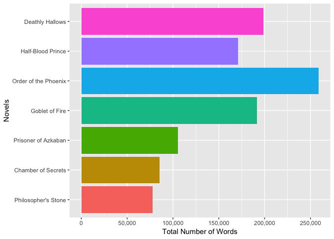
Out of all seven novels, Order of the Pheonix is the longest novels with a total of 258,763 words, while Philosopher’s Stone is the shortest with only 77,875 words.
Next, we’ll list the top ten most commonly used words within all seven novels.
series %>%
  count(word, sort = TRUE) %>%
  top_n(10) # limits output to top 10 results

  A tibble: 10 x 2
    word      n
    <chr> <int>
  1 the   51593
  2 and   27430
  3 to    26985
  4 of    21802
  5 a     20966
  6 he    20322
  7 harry 16557
  8 was   15631
  9 said  14398
  10 his  14264
To no surprise, the most common words include “the”, “and”, “to” “of” and “a”. These are referred to as stop words. This information isn’t very useful as within any novel, as they provide no context. Luckily, there is a function that removes stop words from the tibble.
series %>%
  anti_join(stop_words) %>% # removes all stop words from all novels within series
  count(word, sort = TRUE) %>%
  top_n(10) # limits output to top 10 results

  A tibble: 10 x 2
    word           n
    <chr>      <int>
  1 harry      16557
  2 ron         5750
  3 hermione    4912
  4 dumbledore  2873
  5 looked      2344
  6 professor   2006
  7 hagrid      1732
  8 time        1713
  9 wand        1639
  10 eyes       1604
The results are much better as now we get a better understanding of the novels. For someone who hasn’t read the novel, they could easily deduce who the main characters are.
We can also extract the top three words by novel using dplyr’s data manipulation functions.
series %>%
  anti_join(stop_words) %>% # removes all stop words
  group_by(book) %>%
  count(word, sort = TRUE) %>%
  top_n(3) %>%
  rename(total_count = n) %>% # renames column to total_count
  arrange(book) # order by chronological order of publication

  A tibble: 21 x 3
  Groups:   book [7]
    book                word     total_count
    <fct>               <chr>          <int>
  1 Philosopher's Stone harry           1213
  2 Philosopher's Stone ron              410
  3 Philosopher's Stone hagrid           336
  4 Chamber of Secrets  harry           1503
  5 Chamber of Secrets  ron              650
  6 Chamber of Secrets  hermione         289
  7 Prisoner of Azkaban harry           1824
  8 Prisoner of Azkaban ron              690
  9 Prisoner of Azkaban hermione         603
  10 Goblet of Fire     harry           2936
    … with 11 more rows
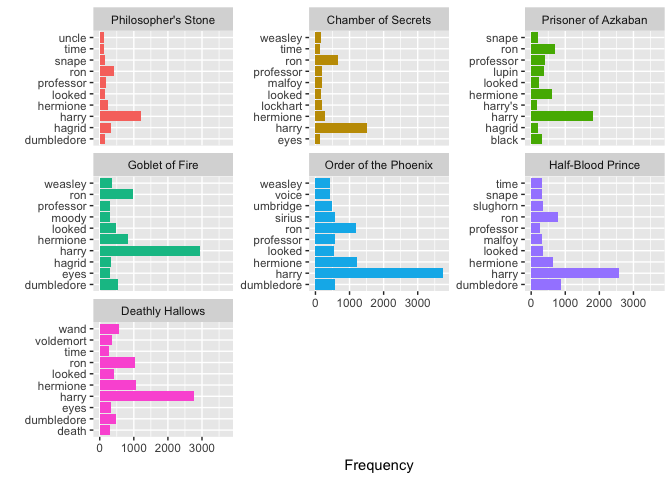
Aside from the Philosopher’s Stone and Half-Blood Prince, the top three words in each novel are Harry, Hermione, and Ron.
Data Visualization
We can visualize the above analysis. Let’s start by plotting the total number of words for each novel.
series %>%
  group_by(book) %>%
  summarize(total_words = n()) %>%
  ungroup() %>%
  ggplot(aes(book, total_words, fill = book)) + # use data from each novel for plot and distinguish novel by color
    geom_bar(stat = "identity") +
    coord_flip() +
    scale_y_continuous(name="Total Number of Words",
                       labels = comma,
                       breaks = c(0, 50000, 100000, 150000, 200000, 250000, 300000)) + # manually set breaks
    scale_x_discrete(name = "Novels") + # sets x axis
    theme(legend.position = "none") # removes legend from plot

Next, we’ll plot the top 10 words used in each novel.
series %>%
  anti_join(stop_words) %>% # remove stop words
  group_by(book) %>%
  count(word, sort = TRUE) %>%
  top_n(10) %>%
  ungroup() %>%
  ggplot(aes(word, n, fill = book)) + # use data from each novel for plot and distinguish novel by color
    geom_bar(stat = "identity") +
    facet_wrap(~ book, scales = "free_y") + # separates plots by novel, "free_y" shares scales across the y-axis
    labs(x = "", y = "Frequency") + # set x and y-axis labels
    coord_flip() + # Flip cartesian coordinates so horizontal becomes vertical vice versa.
    theme(legend.position="none")

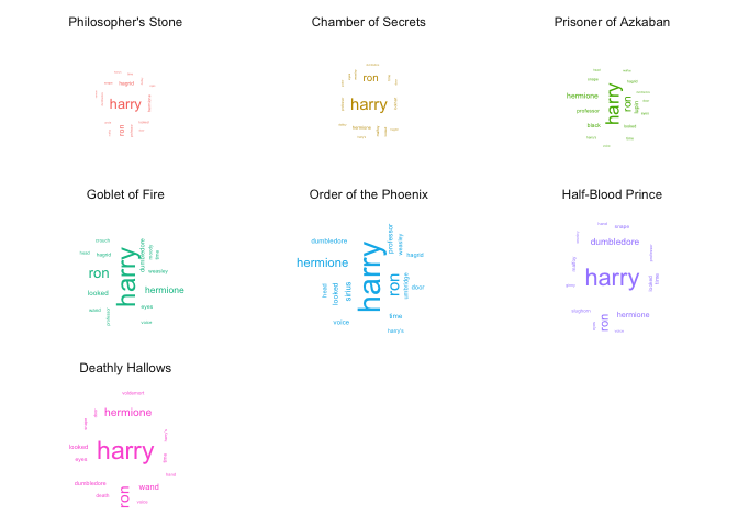
Finally, generating word clouds is another useful way to visualize the frequency of words by novel.
set.seed(123) # for replication purposes
series %>%
  anti_join(stop_words) %>% # remove stop words
  group_by(book) %>%
  count(word, sort = TRUE) %>%
  top_n(15) %>%
  mutate(angle = 90 * sample(c(0, 1), n(), replace = TRUE, prob = c(60, 40))) %>%
  ggplot(aes(label = word,
          size = n,
          color = book,
          angle = angle
    )) +
    geom_text_wordcloud_area(area_corr = TRUE,
        eccentricity = 2) +
    scale_size_area(max_size = 7.5) + # scales the size of the word clouds
    theme_minimal() +
    facet_wrap(~book) # seperates plots by novel

Conclusion:
Getting started on text mining and analysis is quick and easy! If you’re interested in performing simple text analysis on other text, you can install the gutenbergr package. This package provides access to a wide selection of public domain texts. Be on the look out for a future post on sentiment analysis!


