Harry Potter and the Analysis of Text Part 2
The magic of sentiment analysis!
Introduction
Previously we explored how to format text data into tidy text for basic analysis using J.K. Rowling’s Harry Potter series in this post. Today we’ll learn how to perform a more in depth sentiment analysis.
Sentiment analysis involves understanding the opinion or emotion within text. This is achieved by using lexicons. Lexicons are based on unigrams and contain English words that are each assigned a score for positive/negative sentiment as well as emotions such as joy, anger, sadness, etc.
This post will use three lexicons to determine sentiment/emotion of text. These include:
AFINN, a lexicon that assigns words with a score between -5 and 5, with negative scores indicating negative sentiment and positive scores indicating positive sentiment.Bing, a lexicon that categorizes words in a binary fashion into positive and negative categories.NRC, a lexicon that also categorizes in a binary fashion into categories of positive, negative, anger, anticipation, disgust, fear, joy, sadness, suprise and trust.
Step 1: Download the Harry Potter series.
if (packageVersion("devtools") < 1.6) {
  install.packages("devtools")
 }

devtools::install_github("bradleyboehmke/harrypotter", force = TRUE) # provides the first seven novels of the Harry Potter series
Step 2: Load the necessary packages
library(tidyverse)  # loads multiple useful packages
library(harrypotter) # loads harry potter novels
library(tidytext) # provides additional text mining functions
library(ggwordcloud) # provides a word cloud text geom for ggplot2
library(scales) # provides added functions for data visualization
Step 3: Format, clean and tidy the text data
It’s important to remember text data should be properly formatted into a tidy format before starting any analysis, including sentiment analysis.
# store the title of each novel within a variable
titles <- c("Philosopher's Stone",
            "Chamber of Secrets",
            "Prisoner of Azkaban",
            "Goblet of Fire",
            "Order of the Phoenix",
            "Half-Blood Prince",
            "Deathly Hallows")

# all novels will be stored in a large tibble consisting of smaller tibbles for each novel, therefore, format as a list object to store a tibble for each novel
books <- list(philosophers_stone,
                chamber_of_secrets,
                prisoner_of_azkaban,
                goblet_of_fire,
                order_of_the_phoenix,
                half_blood_prince,
                deathly_hallows)


series <- tibble() # create an empty tibble to store the text data

# for loop to unnest and create a tidy text tibble for each novel
for(i in seq_along(titles)) {

  clean <- tibble(chapter = seq_along(books[[i]]),
                  text = books[[i]]) %>% # creates a tibble containing each chapter for each novel
                  unnest_tokens(word, text) %>% # unnests each word to create a 2 column table, with each row containing a single token (word/character) and the chapter it pertains to
                  mutate(book = titles[i]) %>% # adds a third column to identify which novel each token pertains to
                  select(book, everything()) # reorders the columns within the tibble with book as the first column

  series <- rbind(series, clean) # binds the tibble of each novel by rows
}
Step 4: Sentiment Analysis
Overall Sentiment
Once the text data has been cleaned and properly formatted, we can begin sentiment analysis with the NRC lexicon by using the get_sentiments function.
series %>%
  right_join(get_sentiments("nrc")) %>%
  filter(!is.na(sentiment)) %>% # removes tokens that had no sentiment attached
  count(sentiment, sort = TRUE) # retrieves the total count of token for each sentiment
The table below shows the total presence of each sentiment within all the novels.
 A tibble: 10 x 2
    sentiment        n
    <chr>        <int>
  1 negative     56579
  2 positive     38324
  3 sadness      35866
  4 anger        32750
  5 trust        23485
  6 fear         21544
  7 anticipation 21123
  8 joy          14298
  9 disgust      13381
 10 surprise     12991
Sentiment Analysis by Indexed Novel
Next, we can index each novel and create a table that tracks the sentiment as the novel progresses from start to finish. The first step involves indexing the novel, which in this case will be done by every 500 words. Once the novel is indexed, use the Bing lexicon and obtain the positive vs negative sentiment of each index.
series %>%
bing_sentiment <- series %>%
  group_by(book) %>%
  mutate(word_count = 1:n(),
          index = word_count %/% 500 +1) %>% # index each novel by 500 tokens
  inner_join(get_sentiments("bing")) %>%
  count(book, index = index, sentiment) %>% # count the total number positive/negative sentiment
  ungroup() %>%
  spread(sentiment, n, fill = 0) %>% # pivots the data and fills missing data with 0
  mutate(sentiment = positive - negative,
         book = factor(book, levels = titles)) # creates a new variable, sentiment, which is the net count of positive and negative tokens

bing_sentiment %>%
  top_n(-70, index) # limit to the first 10 index of each novel
  A tibble: 70 x 5
    book               index negative positive sentiment
    <fct>              <dbl>    <dbl>    <dbl>     <dbl>
  1 Chamber of Secrets     1       24       12       -12
  2 Chamber of Secrets     2       25       10       -15
  3 Chamber of Secrets     3       11       23        12
  4 Chamber of Secrets     4       16       17         1
  5 Chamber of Secrets     5       20       12        -8
  6 Chamber of Secrets     6       18       13        -5
  7 Chamber of Secrets     7       21       17        -4
  8 Chamber of Secrets     8       28       11       -17
  9 Chamber of Secrets     9       17        7       -10
 10 Chamber of Secrets    10       18       23         5
 … with 60 more rows
The table above shows each novel and it’s index along with the total negative/positive sentiment contained within each index. These negative and positive sentiment scores are summed together to give us the overall sentiment for each index.
Lets repeat the process above using the other lexicons AFINN and NRC.
# Since the afinn lexicon assigns a sentiment value ranging from -5 to 5, we will simply just sum the sentiment value for each index as opposed to using a net difference used in the previous example.
afinn <- series %>%
        group_by(book) %>%
        mutate(word_count = 1:n(),
               index = word_count %/% 500 +1) %>%
        inner_join(get_sentiments("afinn")) %>%
        group_by(book, index) %>%
        summarise(sentiment = sum(value)) %>% # sentiment variable is set up as a sum vs difference
        mutate(method = "AFINN")

# Since both Bing and NRC use a binary classification of positive and negative, we can combine the code and bind the tables
bing_and_nrc <- bind_rows(series %>%
                  group_by(book) %>%
                  mutate(word_count = 1:n(),
                         index = word_count %/% 500 + 1) %>%
                  inner_join(get_sentiments("bing")) %>%
                  mutate(method = "Bing"),
          series %>%
                  group_by(book) %>%
                  mutate(word_count = 1:n(),
                         index = word_count %/% 500 + 1) %>%
                  inner_join(get_sentiments("nrc") %>%
                                     filter(sentiment %in% c("positive", "negative"))) %>%
                  mutate(method = "NRC")) %>%
        count(book, method, index = index , sentiment) %>%
        ungroup() %>%
        spread(sentiment, n, fill = 0) %>%
        mutate(sentiment = positive - negative) %>%
        select(book, index, method, sentiment)

combined_lexicons <- bind_rows(afinn,
                               bing_and_nrc) %>% # bind all three tables
  ungroup() %>%
  mutate(book = factor(book, levels = titles))

combined_lexicons %>%
  top_n(-3, index) %>%
  arrange(book)
 A tibble: 21 x 4
    book                index sentiment method
    <fct>               <dbl>     <dbl> <chr>
  1 Philosopher's Stone     1        11 AFINN
  2 Philosopher's Stone     1         0 Bing
  3 Philosopher's Stone     1         3 NRC
  4 Chamber of Secrets      1       -14 AFINN
  5 Chamber of Secrets      1       -12 Bing
  6 Chamber of Secrets      1       -19 NRC
  7 Prisoner of Azkaban     1        -7 AFINN
  8 Prisoner of Azkaban     1        -7 Bing
  9 Prisoner of Azkaban     1       -11 NRC
 10 Goblet of Fire          1       -22 AFINN
 … with 11 more rows
Similar to the previous table, we are able to see the overall sentiment for each index within each novel and its respective lexicon method used. Notice the different values each lexicon assigns to the same index. Although different in values, the lexicons are pretty consistent in having either a positive or negatice score.
Step 5: Visualizing Sentiment Analysis
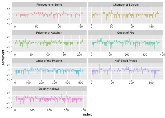
Let’s take it a step further and visualize the sentiment of each novel as it progresses. Using the Bing lexicon and the table we created earlier, we can graph the sentiment on the Y-axis, the index on the X-axis and then facet the graph so each novel has its own visualization for easy comparison.
bing_sentiment %>%
  ggplot(aes(index, sentiment, fill = book)) +
    geom_bar(alpha = 0.5, stat = "identity", show.legend = FALSE) +
    facet_wrap(~ book, ncol = 2, scales = "free_x") # splits the graphs by novel

Based on the visualization from the graphs above, we can easily see how each novel’s sentiment changes as the story progresses. For example, Half-Blood Prince starts with a considerable amount of negative sentiment. Surprisingly, towards the finale of the series in Deathly Hallows, the sentiment remains negative.
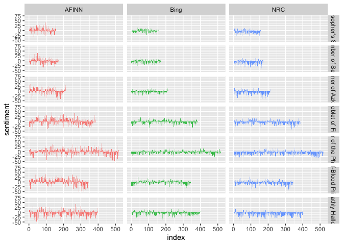
For better comparison among each of the lexicons for the same novel, we can visualize the sentiment similarly above with a slight adjustment and facet the graphs by both lexicon and novel.
combined_lexicons %>%
  ggplot(aes(index, sentiment, fill = method)) +
  geom_bar(alpha = 0.8, stat = "identity", show.legend = FALSE) +
  facet_grid(book ~ method) # split the graphs by each lexicon and by book

Based on the above results, similar peaks and dips in sentiment occur across each of the lexicons with differences on the magnitude of sentiment; the AFINN lexicon tends to have higher degrees of both positive and negative sentiment compared to both Bing and NRC.
Sentiment analysis has endless possibilities and is not limited to novels. Any text document can be analyzed for sentiment including songs, legal documents or social media posts, however, the models may need to be adjusted and the data itself may require further preparation. Regardless, sentiment analysis provides a great opportunity to learn more advanced coding techniques involving data cleaning, text manipulation, and visualization!


